In my post on passive strategies and simple box modeling, I showed how sensitivity analysis can be used to identify the most important passive strategies while still in the pre-design phase. In this post, I’ll show in depth how I did that analysis.

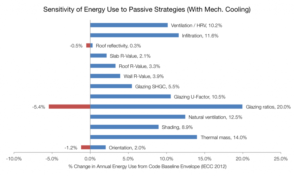
For reference, here is the end product: graphs showing the potential impact of a number of individual strategies.

To do this study, I used Sefaira Architecture for analysis, and used Excel to capture the data and create the graphic. You could get similar data from any energy analysis software, but Sefaira is particularly quick for this type of study. (Full disclosure: I was a Product Manager at Sefaira for several years, so I’m clearly biased.)

Step 1: Select the Variables to Study

I picked primarily envelope variables and passive design strategies — insulation, thermal mass, natural ventilation. However, if I were to do this study again, I would focus more on form and geometry — factors like surface-area-to-volume ratio, floor-to-floor heights, and glazing location on a facade-by-facade basis. Space layout should be on this list, too, especially for buildings that have many different space types within them. These elements all represent critical design decisions that are made very early in design, and more granular insight would have been beneficial.

Step 2: Pick the Right Metric(s)

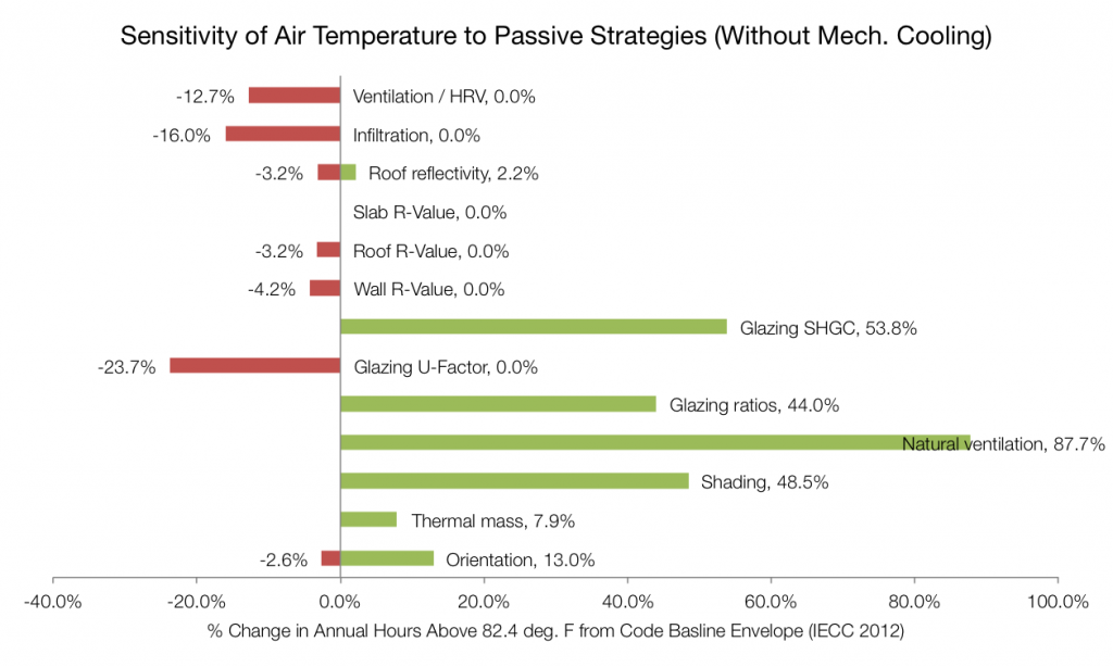
I did the sensitivity study twice: once looking at the impact of each variable on annual energy use, and once looking at the impact on air temperature, assuming no mechanical cooling. The reason was that we were already considering whether we could avoid air conditioning entirely, and I wanted to know what strategies would have the biggest impact on temperatures.

However, I’ve come to believe that annual energy use is not necessarily the best metric to use to inform design. Some strategies, such as shading, may have a small impact on the overall energy, but have a big impact on the peak cooling loads or thermal comfort in a specific space. Reducing that peak load could mean a smaller, cheaper HVAC system, or more HVAC options. For this reason, if I did this analysis again, I would look at impact on peak heating and cooling loads in addition to annual energy use.

Another metric I plan to explore more in the future is Thermal Autonomy — essentially, the percentage of occupied hours in which the space stays comfortable without mechanical systems. I think this has great potential as an early design metric that really highlights passive design.

Step 3: Set up a Baseline

In order to look at the percentage change for each variable, we need some sort of baseline to compare it to. There are several components to a baseline; here’s how I approached each one:

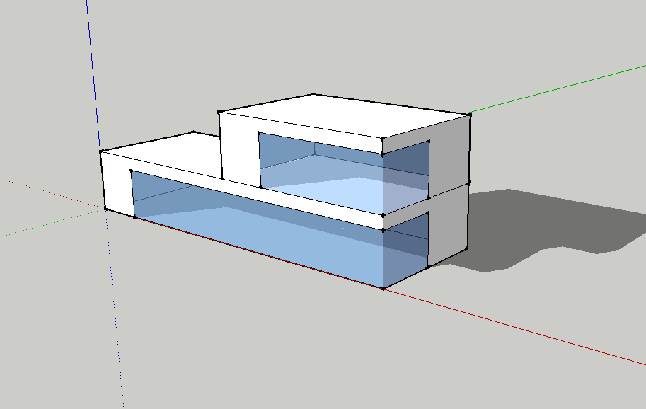
• Building form: I took a rough pass at form based on site constraints and instinct regarding the final design. An alternate approach, particularly if one is studying surface-area-to-volume ratio, is to start out with something “average”: a rectangular shape of middling compactness.
• Glazing ratio: You could use something fairly standard, like 40% glazing on each facade. In this case, I didn’t feel that would be representative of the design, which I expected would have more glazing on the south and almost none on the west — so I took an initial pass at amounts that began to approximate what I would design.
• Envelope properties & construction: I used prescriptive values from the applicable energy code, IECC 2012. In some cases this required calculations to translate from the code value to the model input — for instance, the code specifies a minimum “cavity” R-value; I had to convert this to an overall “assembly” R-value, using standard assumptions about framing dimensions and spacing. In cases where the code was silent — for example, there was no requirement related to glazing solar heat gain coefficient (SHGC) — I chose a typical industry value.

Step 4: Determine Max and Min Values

Next, for each variable, determine the maximum and minimum value to study. These should represent “best case” and “worst case” scenarios for each variable. In many cases the “worst case” was the same as the baseline, since you’re not allowed to be worse than code. The “best case” was determined by either (a) sensitivity analysis using a feature called Response Curves in Sefaira, and/or (b) setting an upper bound based upon what’s technically feasible.

Let’s look at a few examples.

Wall R-Value

The “worst case” value was determined by the minimum prescribed in the energy code: cavity insulation of R-20, which translates to an assembly R-value of 16 if you assume standard framing.

The “best case” was determined by both analysis and technical feasibility. The most super-insulated houses have a wall R-value around R-60 — and these houses end up with walls on the order to 18-24” thick. Anything above this was deemed impractical. I then did a sensitivity analysis to see whether there was an optimum within this range (R-16 to R-60).

Why do analysis? Because many variables behave non-linearly: more insulation is not always better.

Why do analysis? Why not just set the “best case” value to R-60? Because many variables behave non-linearly: more insulation is not always better. In one memorable example, I was working with an architect on an office design, and he wanted to increase the roof insulation as an energy-saving strategy. But when we got aggressive on the insulation, energy use actually increased. This was because the office was cooling-dominated and internally-loaded — laden with heat-generating equipment, people, and lights. Adding insulation just trapped this heat inside the building and increased the cooling load. But the answer was neither “no insulation” — that would have resulted in a ridiculous heating load. The optimum turned out to be be somewhere in the middle. This is why parametric analysis like Sefaira’s Response Curves are so powerful: they provide a fast way to find these local optima.

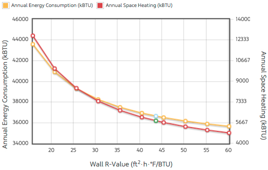
In this case, added insulation showed diminishing returns: anything beyond R-60 would not have had much impact. So R-60 was the “best case.”

Shading

This was a case where analysis determined both the best and worse cases: I used Response Curves to find box the max. and min. values for a horizontal shading device. The worst was zero shading; the best case was an 8-foot overhang.

You might say “That’s obviously impractical! Why didn’t you limit this based on ‘technical feasibility’?” Because the point of this exercise is to highlight the potential impact of shading, not to suggest a solution. If we have this data in early design, we can find creative ways to get an 8-foot-equivalent shade — by incorporating a porch, for example, or a slatted screen that achieves a similar shading ratio. It’s a delicious design challenge, and an excellent example of the value of this exercise.

Building Form

I didn’t actually do this study, but I should have. Here’s what I would have done: I would have create a number of simple box models, each with the same square footage and glazing ratios, but with different degrees of compactness. A perfectly compact form is a sphere; but a cube is a fair approximation. I would then create increments between that shape and a long, thin rectangle. Analyzing each would have produced a max. and min. value for adjusting building form alone.

Step 4: Log data & visualize

I tracked the results of these studies in the Excel sheet shown below. You’ll see results for both annual energy use and air temperature — this required running each analysis twice, with different settings, since one assumed mechanical cooling and the other did not.

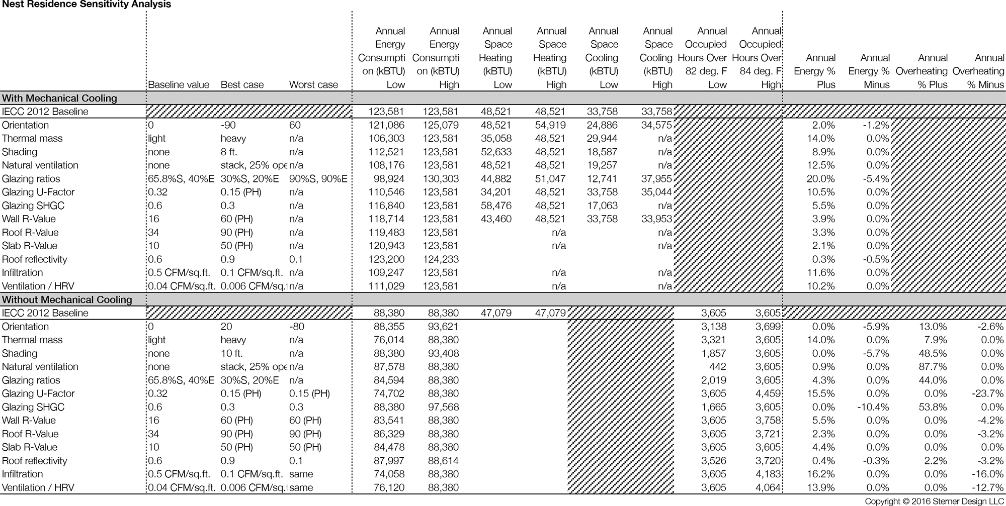
In the final columns of the spreadsheet, I converted the data to a percentage change from the baseline, since the primary concern was relative impact. From this data, I created the final bar charts.

A Note of Caution

Single-variable optimization can find local optima but miss global optima. As I noted in my passive strategy post, combinations of variables are what really matter. The right combination can unlock even greater energy savings, or radically shift the economics of the design — what Amory Lovins calls “tunneling through the cost barrier.” For example, the payback on excellent windows is probably uneconomically long; same with superinsulation and many of the other strategies that we ultimately employed. But with the right combination of strategies, we could eliminate the cooling system, and use a smaller, cheaper heating system — meaning that the combined economics and combined energy savings are actually much better than the individual components by themselves.

The right combination can unlock even greater energy savings, or radically shift the economics of the design.

Similarly, many variables simply can’t be optimized in isolation. Glazing ratios, for instance, should be determined in combination with shading, thermal mass, and glazing properties. More glazing, if considered in isolation, is almost always a liability: it lets heat out in the winter and increases solar gain in the summer. But if we assume optimal shading and thermal mass, or if we change the window properties, the equation changes radically, and we may find that more glass is actually beneficial.

But that’s okay. This analysis is intended only as a starting point — as a way of identifying the “high impact strategies” given our climate, building program, and site, in order to keep them in the front of our minds in early design and begin to integrate them into our thinking going forward. We will follow this analysis with combinatory analysis, like the “passive solar” example I described above, and with more refined optimization later in design.