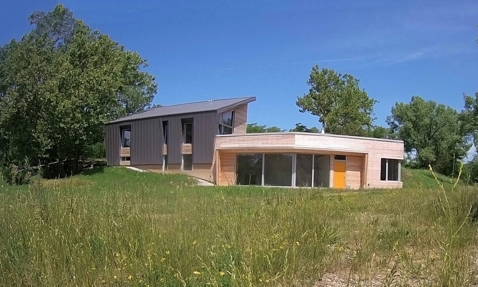
As of August 2022, we have been monitoring energy use at the Iowa Nest Residence for three years post-occupancy. How is the home doing? How does it compare with our predictions and energy models? What lessons can we learn to apply to future ultra-low-energy designs? This post reviews the data and shares some observations and lessons learned.
TL;DR: Key Stats
- The home uses 74% less energy than a conventional new home. If “extra” plug loads (e.g., workshop & servers) are removed, the home uses 90% less than a conventional new home, and 56% LESS than predicted. And all of this is before adding solar panels.
- Heating and cooling loads are 92% less than a conventional home, and 44% less than predicted. This speaks to the success of the passive design strategies.
- Measured energy use is, on average, within 17% of predicted, and the most recent year’s energy use is within 4% of predicted.
- Plug loads (plug-in appliances and equipment) are four times higher than predicted, in part because of a workshop and servers that were not factored into the design-stage energy model.
Provisos and Assumptions
A few things to know about the data:
Servers: The largest wild card in monitored performance was a large server that was located in the home during the first year, which consumed significant energy and put off a significant amount of heat. Because of this, the first year’s data is not representative of typical performance. For this analysis, I’ve either removed this server, or ignored the first year’s data entirely. (See the Appendix to this post for more on my methodology.) The most recent two years of data are both much closer to predicted values, and more consistent with one another.
Weather: The monitored data has NOT been normalized to reflect actual weather conditions. The design-stage energy model used “Typical Meteorological Year” (TMY) weather data; and actual weather always diverges from this typical data–even before including the effects of climate change. A true apples-to-apples comparison would account for this divergence, by normalizing the monitored data based upon actual weather, which I’ve not yet had time to do.
Dehumidification: The home was designed without air conditioning. It was discovered that dehumidification, at least, was necessary to maintain comfort. However, because this had not been installed from the beginning, it was not separately monitored like most other major loads, and shows up in the raw data as a plug load in the basement/workshop area. I have disaggregated the dehumidification based upon the equipment specifications, monitored humidity data, and info from the owners regarding how the equipment was used. But know that this disaggregation is still an estimate — albeit one that does not affect the total energy use figures.
Occupancy: The monitored time period overlaps with COVID-19 and the associated lockdowns, school and office closures, and general disruption to normal patterns of daily life. These disruptions inevitably translate to significant divergence in occupancy and usage patterns compared to “normal” residential patterns. I’ve not attempted to adjust for these changes, but they are worth keeping in mind.
Solar: We contend that it is key to measure in-situ energy use prior to installing solar panels, so that the system is sized for actual rather than theoretical usage. The monitored data described herein will be used to size the system, which will bring the home to Net Zero energy.
The Data
Below are several ways to look at the data. I’ve annotated each chart to explain what it’s showing.
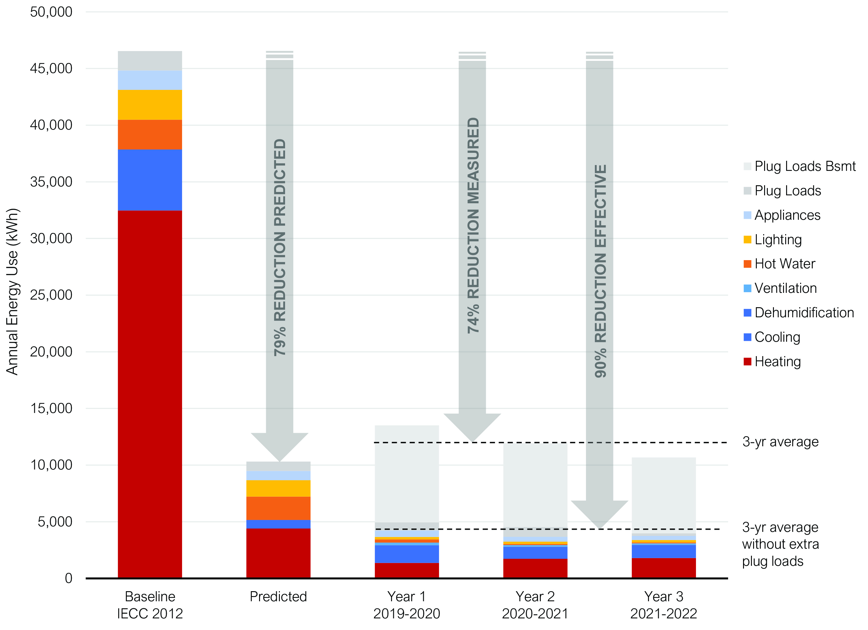
FIG 1: Energy Use vs. Baseline: Here is the overall energy use for all 3 years, compared to both the predicted energy use from the design-phase energy model and the baseline energy use of a conventional new home. The home was predicted to use 79% less energy than the baseline; the average measured reduction is 74%; and the average effective reduction (subtracting the extra plug loads that are not represented in the baseline model) is 90%.
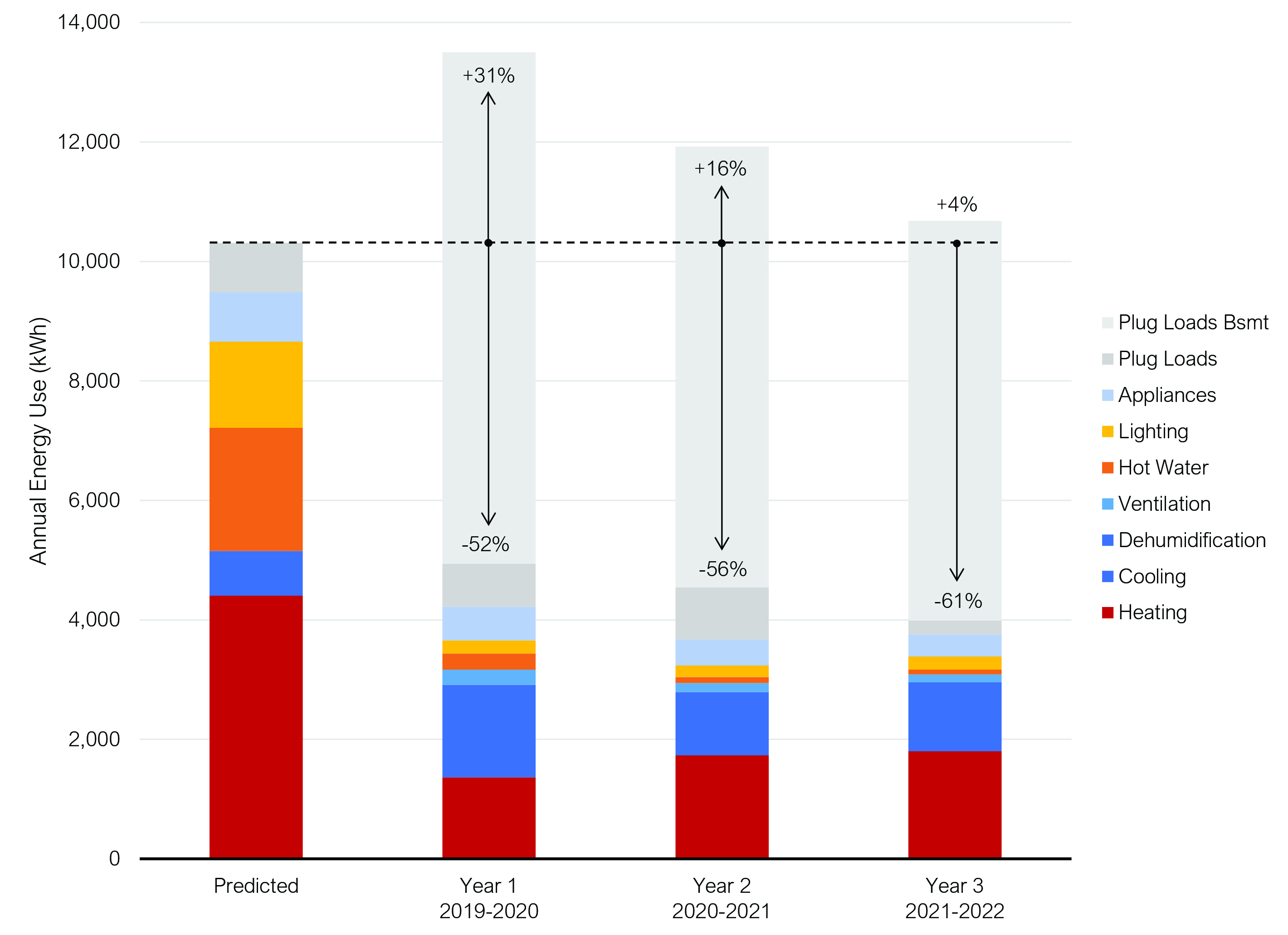
FIG 2: Energy Use vs. Predicted: Here’s how measured performance stacks up to predicted. The three-year average energy use is 16% higher than predicted. The first year was 31% higher than predicted, and the most recent year was 4% higher. The distribution of the energy use, however, is significantly different than predicted: heating and cooling are roughly 44% less than predicted; lighting and hot water are likewise significantly less than predicted; and plug loads are on average 4 times higher than predicted. Note that the majority of these plug loads, identified as “Plug Loads Bsmt” in the charts, are from a workshop and servers that were not included in the original analysis. If these loads are ignored, the actual energy use is between 52% and 61% LESS than predicted.
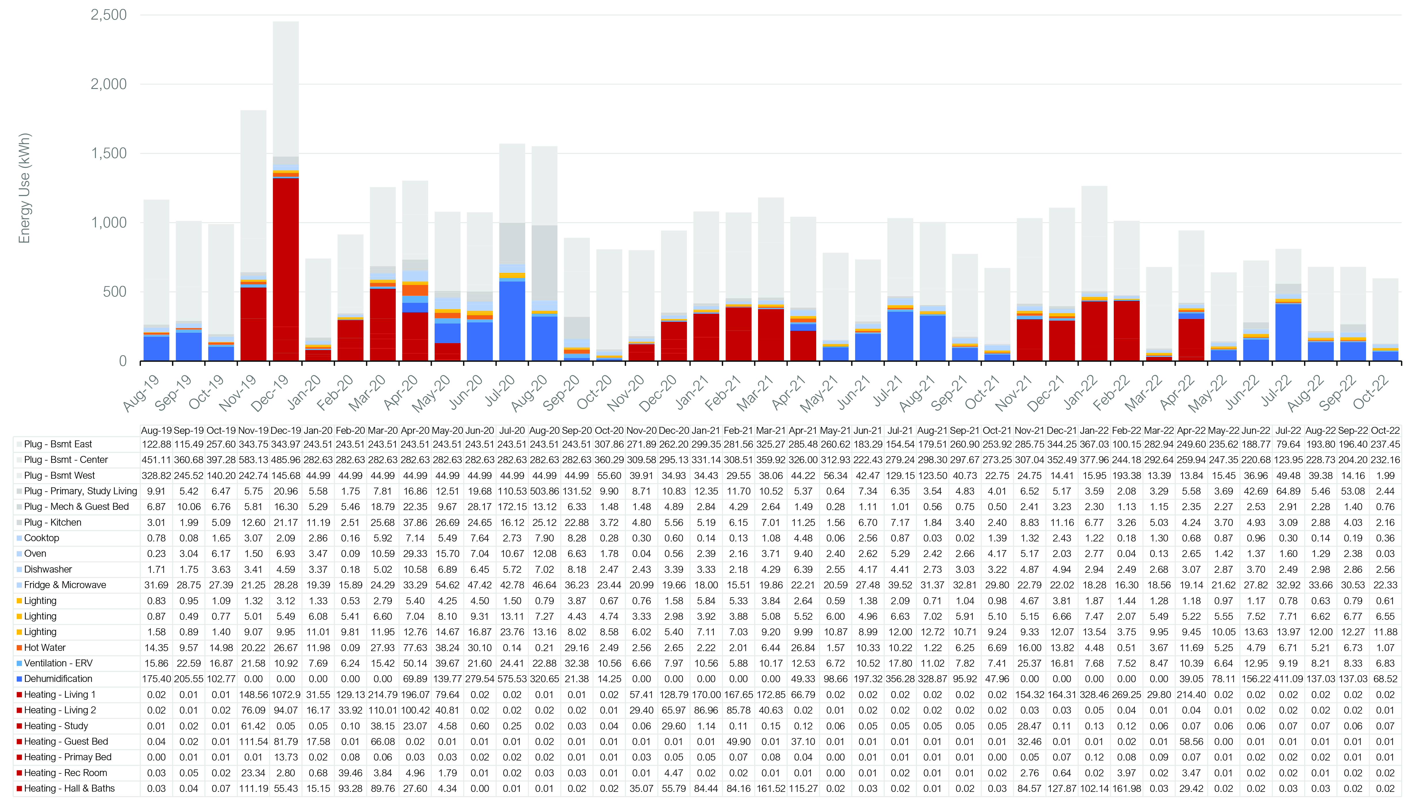
FIG 3: Monthly Energy Use: This is for the energy nerds who want to really dig into the data. It shows energy use for each zone on a month-by-month basis. As expected, heating and dehumidification follow seasonal patterns, and plug loads are relatively constant. The first year shows higher monthly variability than subsequent years (more on this later).
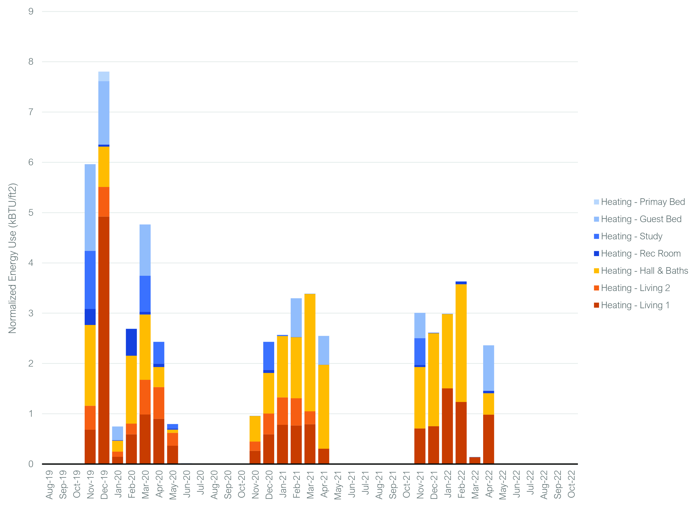
FIG 4: Monthly Heating Energy Use by Zone: This chart shows normalized (per square foot) heating energy use on a zone-by-zone basis for each month. Living areas (orange), on average, use the most heat per square foot; followed closely by the bathrooms (yellow). Bedrooms are the lowest. Overall, the home uses just 1.89 kBTU/ft2/yr on average for heating. In a heating dominated climate like Iowa, one would expect the average home to use ~30kBTU/ft2/yr; and the Passive House Heating Demand target for this home is 10 kBTU/ft2/yr.
Observations and Lessons Learned
1. Passive design works — really well! Heating and cooling loads are minuscule—92% less than the conventional baseline, and 44% less than predicted . Heating requires just 1.89 kBTU/ft2/yr, and cooling (dehumidification) approximately 1.45 kBTU/ft2/yr—lower, in fact, than most Passive Houses. The passive design measures employed here worked, and worked better than expected.
2. Energy modeling is essential, even when not perfectly predictive. Early-stage Sefaira energy models gave important—indeed, essential—guidance on the key factors driving energy use, and the monitored data bears out the impact of these strategies. We would not have been able to achieve this level of performance without early performance analysis.
3. Zoned radiant heating is awesome. Even normalized for square footage, the heating energy use of different zones varies widely (see Fig 4 above). Importantly, the variation does NOT appear to be related to exposed surface area or the amount of glass—instead, it appears to reflect usage and comfort preferences, given the homeowner’s ability to set thermostats independently in each zone to provide heat only where and when they need it. This is predominantly in the living areas and bathrooms (who doesn’t love a warm floor after a shower?). The bedrooms do not use much heat—likely because most people prefer cooler temperatures for sleeping. Homeowners reported setting underfloor set points in winter to 65F (bedrooms) and 68F (bathrooms). This ability to fine-tune heating not only creates a delightful and varied thermal experience—it’s also another reason for the minuscule heating energy use.
4. Plug loads were significantly under-estimated. The plug loads were far higher than expected—specifically for the basement, which included a workshop and servers that had not been factored into the original model. (These loads were high even when the largest server was removed.) These additional appliances also generate more heat, which may partially explain the lower heating loads. Early-stage plug load estimates may need to be more conservative, and special uses clearly discussed early in design. (Note that Phius has developed useful calculators for estimating “Miscellaneous Electrical Loads,” which would likely have led to a more conservative / accurate estimate—but were not available at the time this home was being designed.)
5. Hot water was significantly overestimated. The home has a super-efficient condensing washer, ultra-low-flow Nebia showerheads (0.72 gallons per minute vs 2.0+ for conventional), a very compact plumbing system with less than 100 linear feet of total Pex length (that therefore loses very little heat), and an instantaneous water heater that only produces hot water when needed. Together these yielded hot water energy use 93% less than the already-conservative prediction. The owners also deserve credit, as water use is heavily influenced by the occupant’s usage patterns. (My grandmother, for instance, used to leave the hot water running while cleaning up after dinner—a process that included pre-washing the dishes before they went into the dishwasher. If she lived here, the numbers would look very different.)
6. Lighting was significantly overestimated. This is likely due in part to the excellent daylighting, which makes electric lighting unnecessary for much of the day. Credit was not taken for daylight in the early-stage energy models—which is typical practice, but also clearly resulted in over-estimated lighting demand.
7. It’s hard to avoid cooling—especially in a humid climate like Iowa. While the home still has no conventional cooling system, it does have a dehumidifier, which turned out to be necessary to maintain comfort (and avoid mold and mildew). The dehumidifier is set in the basement and tunnel areas, and keeps those areas in the 38-45% RH band. The resulting cooling loads are slightly higher than predicted, though still lower than a conventional home—however, this number is largely an estimate (described more fully in the appendix below) and may be overstated. It’s also possible that the higher than predicted value is accurate, and due in part to the hotter and more humid summers that Iowa has been experiencing as a result of climate change—a trend not captured in the historically-based TMY (Typical Meteorological Year) weather files.
8. There is a learning curve for operating the home. The first year’s energy use is “spiky”—particularly the radiant heating—with high variability and extremes not seen in the subsequent years. Likely the homeowners were getting used to how to control the home’s unique systems to maintain comfort—particularly given the thermal lag inherent in the thermally massive concrete floor.
My key takeaway is this: the home’s passive design strategies are working—if anything, better than predicted.
Appendix – Notes on Methodology
Methodology for Estimating Dehumidifier Energy Use
As discussed above, the dehumidifier was not monitored separately, and shows up in the basement plug loads. Here’s how I disaggregated it:
- Sourced historical daily Temperature and Relative Humidity data from Visual Crossing for the relevant zip code for the timeframe, https://www.visualcrossing.com/weather/weather-data-services
- Used the “Calculator for Dehumidification Energy Load” by Tim Padfield, available at: https://www.conservationphysics.org/atmcalc/dehumidcalc.htm, which estimates dehumidifier energy used based upon outdoor temperature and humidity, indoor setpoints, air leakage, and cellulose buffer capacity. Air leakage was taken from blower door tests; cellulose capacity was estimated but had a negligible effect on results.
- The results were equivalent to running a 300W dehumidifier for approximately 50% of hours annually.
- The period from May-September 2020 was increased to 1.5x the estimated to reflect additional dehumidification of the garage during this period, due to a very wet summer.
- Subtracted the resulting energy on a monthly basis from the total Plug Load and added it to its own category (Dehumidification); total energy use remained unchanged.
Methodology for Estimating Basement Lighting Energy Use
Basement lighting was not separately monitored; it shows up in the total basement plug loads. Here’s how I disaggregated it:
- Calculated per-square foot lighting energy use for the Rec Room, which was judged to be the most similar zone, as it has lower occupancy rates and limited daylighting.
- This per-square-foot factor was applied to the basement area.
- The figure was added to the Lighting category and subtracted from the basement plug loads; total energy use remained unchanged.
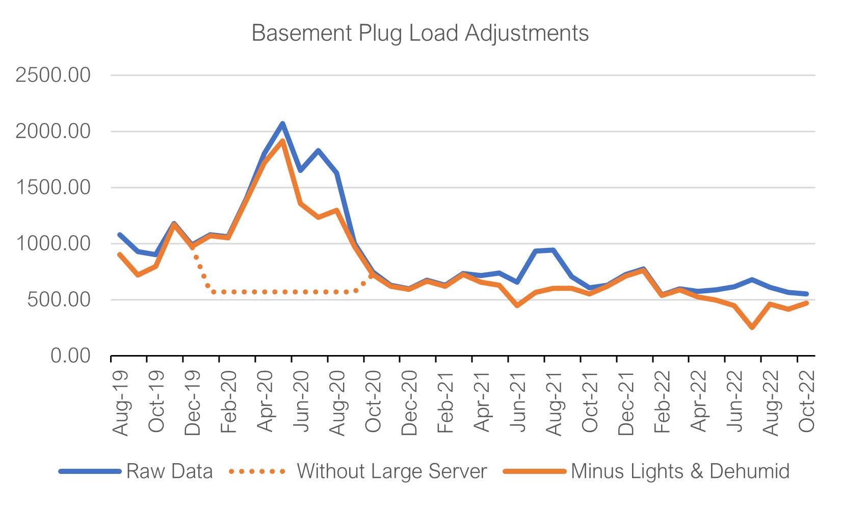
Methodology for Removing Large Server
- The large server in question (900 to 1800W) was in service between January and September 2020, and shows up in the data as part of the basement plug loads.
- For this time period, I averaged post-server energy use for the basement plug loads, after removing dehumidification and lighting loads (discussed above). I used this average for the period in question.
- Note that other equipment, including other, smaller servers and tools, remained, and account for the remaining basement plug load consumption, which stands at a relatively constant 400W year-round.
Thanks for sharing this information Peter – really interesting and great to see it’s performing even better than expected 🙂